Solve Manning's Equation with Python Scipy library

from scipy.optimize import root

def manningC(d, args):
    Q, w,h,sSlopeL,sSlopeR,nMann,lSlope = args
    #left side slope can be different from right side slope
    area = ((((d*sSlopeL)+(d*sSlopeR)+w)+w)/2)*d
    # wet perimeter
    wPer = w+(d*(sSlopeL*sSlopeL+1)**0.5)+(d*(sSlopeR*sSlopeR+1)**0.5)
    #Hydraulic Radius
    hR = area/ wPer
    # following formula must be zero
    # manipulation of Manning's formula
    mannR = (Q*nMann/lSlope**0.5)-(area*hR**(2.0/3.0))
    return mannR
    
###### MAIN CODE
# the following are input data to our open channel manning calculation
# flow, width, height, left side slope, right side slope, 
# Manning coefficient, longitudinal slope
args0 = [2.5,2,.5,1.0,1.0,.015,.005]
initD = .00001  # initial water depth value

# then we call the root scipy function to the manningC
sol =root(manningC,initD, args=(args0,))    
# print the root found
print(sol.x)

Pandas sum column values according to another columns value

One-liner code to sum Pandas second columns according to same values in the first column.

df2 = df1.groupby(df1.columns[0])[df1.columns[1]].sum().reset_index()

For example, applying to a table listing pipe diameters and lenghts, the command will return total lenghts according to each unique diameters.

This functionality is similar to excel's pivot table sum.

Multiple linear regression in Python

Sometimes we need to do a linear regression, and we know most used spreadsheet software does not do it well nor easily.

In the other hand, a multiple regression in Python, using the scikit-learn library - sklearn - it is rather simple.

import matplotlib.pyplot as plt
import pandas as pd
from sklearn.linear_model import LinearRegression

# Importing the dataset
dataset = pd.read_csv('data.csv')
# separate last column of dataset as dependent variable - y
X = dataset.iloc[:, :-1].values
y = dataset.iloc[:, -1].values

# build the regressor and print summary results
regressor = LinearRegression()
regressor.fit(X,y)
print('Coefficients:\t','\t'.join([str(c) for c in regressor.coef_]))
print('R2 =\t',regressor.score(X,y, sample_weight=None))

#plot the results if you like
y_pred = regressor.predict(X)
plt.scatter(y_pred,y)
plt.plot([min(y_pred),max(y_pred)],[min(y_pred),max(y_pred)])
plt.legend()
plt.show()

A Library to connect Excel with Python - PYTHON FOR EXCEL

PYTHON FOR EXCEL. FREE & OPEN SOURCE.

xlwings - Make Excel Fly!

xlwings is a BSD-licensed Python library that makes it easy to call Python from Excel and vice versa:
Scripting: Automate/interact with Excel from Python using a syntax close to VBA.

- Macros: Replace VBA macros with clean and powerful Python code.
- UDFs: Write User Defined Functions (UDFs) in Python (Windows only).

Numpy arrays and Pandas Series/DataFrames are fully supported. xlwings-powered workbooks are easy to distribute and work on Windows and Mac.

Install with: pip install xlwings;

It is already included in Winpython and in Anaconda.

Links

https://www.xlwings.org/

http://docs.xlwings.org/en/stable/index.html

https://winpython.github.io/

https://www.continuum.io/downloads

Alternating Block Hyetograph Method with Python

To generate hypothetic storm events, we can use some methods as Alternating block method, Chicago method, Balanced method, SCS Storms among others.

In this post I show a way to generate a hypothetic storm event using the Alternating block method.

This python code uses the numpy library. The altblocks functions uses as input the idf parameters as list, and total duration, delta time and return period as floats.

import numpy as np

def altblocks(idf,dur,dt,RP):
    aDur = np.arange(dt,dur+dt,dt)    # in minutes
    aInt = (idf[0]*RP**idf[1])/((aDur+idf[2])**idf[3])  # idf equation - in mm/h
    aDeltaPmm = np.diff(np.append(0,np.multiply(aInt,aDur/60.0)))
    aOrd=np.append(np.arange(1,len(aDur)+1,2)[::-1],np.arange(2,len(aDur)+1,2))
    prec = np.asarray([aDeltaPmm[x-1] for x in aOrd])
    aAltBl = np.vstack((aDur,prec))
    return aAltBl

Make numpy array of 'datetime' between two dates

A simple way to create an array of dates (time series), between two dates:

We can use the numpy arange - https://docs.scipy.org/doc/numpy/reference/generated/numpy.arange.html , function which is most used to create arrays using start / stop / step arguments.

Syntax:
numpy.arange([start, ]stop, [step, ]dtype=None)

In case of datetime values, we need to specify the step value, and the correct type and unit of the timestep in the dtype argument

. dtype='datetime64[m]' will set the timestep unit to minutes;
. dtype='datetime64[h]' will set the timestep unit to hours;
. dtype='datetime64[D]' will set the timestep unit to days;
. dtype='datetime64[M]' will set the timestep unit to months;
. dtype='datetime64[Y]' will set the timestep unit to months;

For example:

import numpy as np

dates = np.arange('2017-06-01', '2017-06-02', 15, dtype='datetime64[m]')
# 15 is the timestep value, dtype='datetime64[m] means that the step is datetime minutes

This example will create an array of 96 values, between 01jun2017 and 02jun2017, with a time step of 15 minutes.

Solving Manning's equation for channels with Python

Manning's equation is a very common formula used in hydraulic engineering. It is an empirical formula that estimates the average velocity of open channel flow, based on a roughness coefficient.



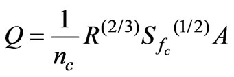
The problem of solving Manning's formula is that it is an implicit formula - the water depth variable (independent variable) is inside R (Hydraulic Radius) and A (flow area) - becoming dificult to isolate the independent variable.

A common approach for solving this equation is to use numerical methods, as the Newton-Raphson method.

In this case, we try different water depths until the function 

 - a manipulation of the original manning formula, became equal to zero.

An implementation for the resolution of the above, for open channels and using the Newton-Raphson approximation, is shown below.

If you found this code of this explanation useful, please let me know. 

def manningC(lam, args):
    Q,base,alt,talE,talD,nMann,decl = args
    area = ((((lam*talE)+(lam*talD)+base)+base)/2)*lam
    perM = base+(lam*(talE*talE+1)**0.5)+(lam*(talD*talD+1)**0.5)
    raio = area/ perM
    mannR = (Q*nMann/decl**0.5)-(area*raio**(2.0/3.0))
    return mannR

def solve(f, x0, h, args):
    lastX = x0
    nextX = lastX + 10* h  # "different than lastX so loop starts OK
    while (abs(lastX - nextX) > h):  # this is how you terminate the loop - note use of abs()
        newY = f(nextX,args)  # just for debug... see what happens
        # print out progress... again just debug
        print lastX," -> f(", nextX, ") = ", newY     
        lastX = nextX
        nextX = lastX - newY / derivative(f, lastX, h, args)  # update estimate using N-R
    return nextX

def derivative(f, x, h, args):
    return (f(x+h,args) - f(x-h,args)) / (2.0*h)

if __name__=='__main__':
    # arguments in this case are - flow, bottom width, height,
    # Left side slope, rigth side slope, manning, longitudinal slope
    args0 = [2.5,1,.5,1.0,1.0,.015,.005]
    initD = .01
    # call the solver with a precision of 0.001
    xFound = solve(manningC, initD, 0.001, args0)
    print 'Solution Found - Water depth = %.3f' %xFound

Python and Pandas - How to plot Multiple Curves with 5 Lines of Code

In this post I will show how to use pandas to do a minimalist but pretty line chart, with as many curves we want.

In this case I will use a I-D-F precipitation table, with lines corresponding to Return Periods (years) and columns corresponding to durations, in minutes. as shown below:

For the code to work properly, the table must have headers in the columns and lines, and the first cell have to be blank. Select the table you want in your SpreadSheet Editor, and copy it to clipboard.

Then, run the following code:

import pandas as pd

table = pd.read_clipboard()
tabTr = table.transpose().convert_objects(convert_numeric=True)
eixox = tabTr.index.values.astype(float)
tabTr.set_index(eixox).plot(grid=True)

And Voila!:

Reading Text files in Python

This is a basic funcionality, but very useful for many applications.

It opens a pure text file. You do not have to import any extra library.

The main sintax for opening files is:

file_object = open(file_name [, access_mode][, buffering])

where:
file_object -> variable
file_name -> the file you want to open
access_mode -> 'r' for read, 'rw' for read and wite text files
buffering -> size of data you read from file. If you leave this blank, it uses the system default - recommended.

To read only text files, it becomes:

file = open('yourfile.txt', 'r')

'yourfile.txt' must contain the correct folder address to it.
'r' stands for read only.

If you want all the contents of your file in one string, you can call read() method:

print file.read()

A good way to deal with text files is to turn the text into a list, each line as an list element. To do this, use the readlines() method:

lstLines = file.readlines()

After all the readings and processings you want to do with the file, you have to close it as following:

file.close()

How to use active layer in QGIS python - PyQGIS

Just use the activeLayer() as in the following code.

mylayer = qgis.utils.iface.activeLayer()
print mylayer.name(), " - ",mylayer

SWMM5 in Python !

Do you use SWMM5?

Have you already wanted some nicer output?
Or some kind of presentation of results that the programs does not fit you?

So, you might be interested in the SWMM5 package for python

https://pypi.python.org/pypi/SWMM5

It gathers all information from .INP files, letting you to play with all the components and the results.

How to install:

If you have already installed pip , just open OSGEO4W and type:

pip install SWMM5

If QGIS is opened, you will have to restart it.

Documentation and examples are included in the website given.

Installing pip in PyQGIS

"pip" is a package management system used to install and manage software packages written in Python. Many packages can be found in the Python Package Index (PyPI).

Many modules are installed through "pip", so as the SWMM5 module.

Installing pip in QGIS - python - PyQgis - OSGeo4w

1 - Download pip - https://bootstrap.pypa.io/get-pip.py ;
2 - Open OSGeo4W;
3 - go to the get-pip.py folder and type:
python get-pip.py

How to Install New Python Modules / Packages in QGIS - method #1

Steps:


1 - copy source folder to C:\Program Files\QGIS Wien\apps\Python27\Lib\site-packages

2 - Open OSGeo4W Shell; go to unpacked folder, where setup.py lies - (>> cd "C:\Program Files\QGIS Wien\apps\Python27\Lib\site-packages")

3 - Type: >> python setup.py install



-----


If it shows errors regarding setuptools: you will have to install setuptools.


https://pypi.python.org/packages/source/s/setuptools/setuptools-18.4.zip#md5=38d5cd321ca9de2cdb1dafcac4cb7007


Download setuptools package, then repeat the same steps for installation.

Ps: in my opinion, this is the worst method to install modules. Next post I will tell how to use "pip" with QGIS Python.

How to Learn Python

That is how I learned Python:

https://www.codecademy.com/learn/python

Excellent site. Recommended.

Opening Python Editor in QGIS

How to Use Python

In this post I will try to explain how I started using PYTHON to solve everyday work needs.

You can go to Python Official site - https://www.python.org/ - and dowload the latest packages for you operating system:
https://www.python.org/downloads/

----

However, some programs already come with a python console included - that is the case of QGIS (Quantum GIS). That is how I started to code in python - with QGIS -  http://www.qgis.org/en/site/

QGIS is a Open-Source desktop GIS - it is a computer software which is really very useful for hydrologists and hydraulic engineers. And it is continuosly evolving, getting better in every new version. At the time of thise post, the current version is the 2.12 - Lyon.

QGIS has depository of plugins - users make their own plugins and share with the community. And these plugins are all python coded.

QGIS comes with a python console. And with a code editor. And there is where the show begins!!

Upcoming posts will show reference material, screenshots, and a lot of examples.

Thanks for visiting.

About the blog

In this blog I will post all of the codes for scripts or functions that I developed or found interesting, during the development of python scripts for Hydrology and Hydraulics.